Ch. 5 - Integration
Briggs - Calculus: Early Transcendentals 3rd Edition
Briggs3rd EditionCalculus: Early TranscendentalsISBN: 9780136847243Not the one you use?Change textbook
Chapter 5, Problem 5.4.45c

Explain why or why not Determine whether the following statements are true and give an explanation or counterexample.
(c) The average value of a linear function on an interval [a, b] is the function value at the midpoint of [a, b] .

Verified step by step guidance
1
Step 1: Recall the formula for the average value of a function f(x) on an interval [a, b]. It is given by: 1(b-a)abf(x)dx.
Step 2: For a linear function, f(x) = mx + c, substitute this into the formula for the average value. The integral becomes: ab(mx+c)dx.
Step 3: Compute the integral of the linear function. The integral of mx is m2x2, and the integral of c is cx. Evaluate these terms at the bounds a and b.
Step 4: Simplify the result of the integral and divide by (b - a) to find the average value. After simplification, the average value of the linear function will be: m((a+b)2)+c, which is the function value at the midpoint of [a, b].
Step 5: Conclude that the statement is true. The average value of a linear function on an interval [a, b] is indeed equal to the function value at the midpoint of [a, b], as shown by the calculation.

Verified video answer for a similar problem:

This video solution was recommended by our tutors as helpful for the problem above.
Video duration:
4m
Was this helpful?

Key Concepts

Here are the essential concepts you must grasp in order to answer the question correctly.

Average Value of a Function

The average value of a function f(x) over an interval [a, b] is calculated using the formula (1/(b-a)) * ∫[a to b] f(x) dx. This concept is crucial for understanding how to find the mean value of a function across a specified range, which can differ from simply evaluating the function at a single point.
Recommended video:
06:37
Average Value of a Function

Linear Functions

A linear function is a polynomial function of degree one, typically expressed in the form f(x) = mx + b, where m is the slope and b is the y-intercept. The properties of linear functions, such as constant slope and direct proportionality, influence how their average value behaves over an interval.
Recommended video:
07:17
Linearization

Midpoint of an Interval

The midpoint of an interval [a, b] is calculated as (a + b)/2. For linear functions, evaluating the function at this midpoint can yield the average value, but this is not true for non-linear functions. Understanding this concept helps clarify why the statement may hold true specifically for linear functions.
Recommended video:
07:39
Left, Right, & Midpoint Riemann Sums
Related Practice
Textbook Question

Explain why or why not Determine whether the following statements are true and give an explanation or counterexample.

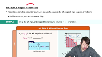
(c) For an increasing or decreasing nonconstant function on an interval [a,b] and a given value of n, the value of the midpoint Riemann sum always lies between the values of the left and right Riemann sums.

1
views
Textbook Question

Properties of integrals Suppose ∫₀³ƒ(𝓍) d𝓍 = 2 , ∫₃⁶ƒ(𝓍) d𝓍 = ―5 , and ∫₃⁶g(𝓍) d𝓍 = 1. Evaluate the following integrals.

(d) ∫₆³ (ƒ(𝓍) + 2g(𝓍)) d𝓍

Textbook Question

Explain why or why not Determine whether the following statements are true and give an explanation or counterexample.                                                                          

                                                                                                                                                                                     (c) The functions p(𝓍) = sin 3𝓍 and q(𝓍) = 4 sin 3𝓍 are antiderivatives of the same function. 

Textbook Question

Use Table 5.6 to evaluate the following definite integrals.                                                                                                                    

 (c) ∫₃√₂^⁶ d𝓍/(𝓍² ―9)

1
views
Textbook Question

Mass from density A thin 10-cm rod is made of an alloy whose density varies along its length according to the function shown in the figure. Assume density is measured in units of g/cm. In Chapter 6, we show that the mass of the rod is the area under the density curve.

(c) Find the mass of the entire rod (0 ≤ x ≤ 10) .

1
views
Textbook Question

{Use of Tech} Approximating definite integrals Complete the following steps for the given integral and the given value of n. 

(c) Calculate the left and right Riemann sums for the given value of n.

∫₁⁷ 1/𝓍 d𝓍 ; n = 6