Textbook Question
Comparing Two Means Treating the data as samples from larger populations, test the claim that there is a significant difference between the mean of presidents and the mean of popes.
1
views
 Verified step by step guidance
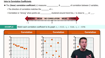
 05:43
05:43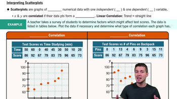 06:36
06:36 4:01
4:01Comparing Two Means Treating the data as samples from larger populations, test the claim that there is a significant difference between the mean of presidents and the mean of popes.
Notation Using the weights (lb) and highway fuel consumption amounts (mi/gal) of the 48 cars listed in Data Set 35 “Car Data” of Appendix B, we get this regression equation:
y^ = 58.9 - 0.00749x, where x represents weight.
c. What is the predictor variable?
Notation The author conducted an experiment in which the height of each student was measured in centimeters and those heights were matched with the same students’ scores on the first statistics test.
c. Does r change if the heights are converted from centimeters to inches?
Exercises 1–10 are based on the following sample data consisting of costs of dinner (dollars) and the amounts of tips (dollars) left by diners. The data were collected by students of the author.
Predictions Repeat the preceding exercise assuming that the linear correlation coefficient is r = 0.132.
Sum of Squares Criterion In addition to the value of another measurement used to assess the quality of a model is the sum of squares of the residuals. Recall from Section 10-2 that a residual is (the difference between an observed y value and the value predicted from the model). Better models have smaller sums of squares. Refer to the U.S. population data in Table 10-7.
c. Verify that according to the sum of squares criterion, the quadratic model is better than the linear model.
Testing for a Linear Correlation
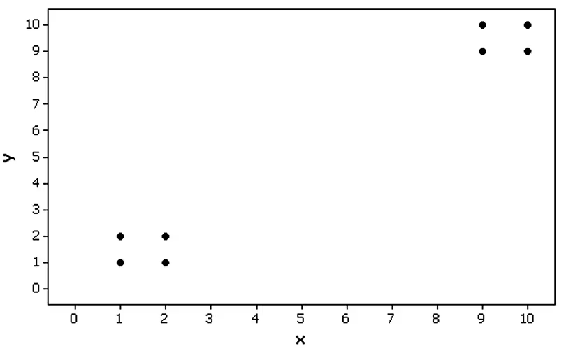
In Exercises 13–28, construct a scatterplot, and find the value of the linear correlation coefficient r. Also find the P-value or the critical values of r from Table A-6. Use a significance level of α = 0.05. Determine whether there is sufficient evidence to support a claim of a linear correlation between the two variables. (Save your work because the same data sets will be used in Section 10-2 exercises.)
Powerball Jackpots and Tickets Sold Listed below are the same data from Table 10-1 in the Chapter Problem, but an additional pair of values has been added in the last column. Is there sufficient evidence to conclude that there is a linear correlation between lottery jackpot amounts and numbers of tickets sold? Comment on the effect of the added pair of values in the last column. Compare the results to those obtained in Example 4.
[IMAGE]