Textbook Question
What conditions are necessary in order to use the z-test to test the difference between two population means?

 Verified step by step guidance
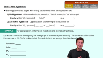
 06:21
06:21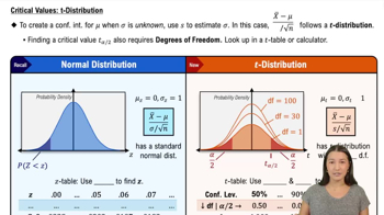 05:50
05:50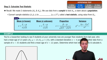 06:34
06:34What conditions are necessary in order to use the z-test to test the difference between two population means?
Test the claim about the difference between two population means and at the level of significance α. Assume the samples are random and independent, and the populations are normally distributed.
Claim: μ1=μ2, α=0.01, Assume (σ1)^2=(σ2)^2
Constructing Confidence Intervals for μ1-μ2. You can construct a confidence interval for the difference between two population means μ1-μ2 , as shown below, when both population standard deviations are known, and either both populations are normally distributed or both n1>= 30 and n2>=30 . Also, the samples must be randomly selected and independent.
[Image]
In Exercises 29 and 30, construct the indicated confidence interval for μ1-μ2 .
Software Engineer Salaries Construct a 95% confidence interval for the difference between the mean annual salaries of entry level software engineers in Santa Clara, California, and Greenwich, CT, using the data from Exercise 27.
[APPLET] Teaching Methods
Two teaching methods and their effects on science test scores are being reviewed. A group of students is taught in traditional lab sessions. A second group of students is taught using interactive simulation software. The science test scores for the two groups are shown in the back-to-back stem-and-leaf plot.
At , α=0.01 can you support the claim that the mean science test score is lower for students taught using the traditional lab method than it is for students taught using the interactive simulation software? Assume the population variances are equal.
Young Adults In a survey of 3500 males ages 20 to 24 whose highest level of education is some college, but no bachelor’s degree, 80.2% were employed. In a survey of 2000 males ages 20 to 24 whose highest level of education is a bachelor’s degree or higher, 86.4% were employed. At α=0.01, can you support the claim that there is a difference in the proportion of those employed between the two groups? (Adapted from National Center for Education Statistics)
In Exercises 11–14, test the claim about the difference between two population means and at the level of significance . Assume the samples are random and independent, and the populations are normally distributed.
Claim: μ1<μ2; α=0.03
Population statistics:σ1=136 and σ2=215
Sample Statistics: x̅1=5004, n1=144, x̅2=4895, n2=156