Textbook Question
25–28. Two steps of Euler’s method For the following initial value problems, compute the first two approximations u1 and u2 given by Euler’s method using the given time step.
y′(t) = 2−y, y(0) = 1; Δt = 0.1
1
views

 Verified step by step guidance
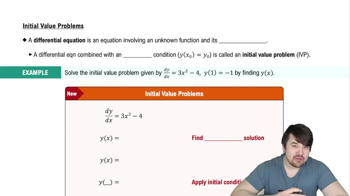
 05:03
05:03 6:04
6:04 06:46
06:4625–28. Two steps of Euler’s method For the following initial value problems, compute the first two approximations u1 and u2 given by Euler’s method using the given time step.
y′(t) = 2−y, y(0) = 1; Δt = 0.1
12–16. Sketching direction fields Use the window [-2, 2] x [-2, 2] to sketch a direction field for the following equations. Then sketch the solution curve that corresponds to the given initial condition. A detailed direction field is not needed.
y(x) = sin y, y(−2) = 1/2
The general solution of a first-order linear differential equation is y(t) = Ce⁻¹⁰ᵗ − 13. What solution satisfies the initial condition y(0) = 4?
5–10. First-order linear equations Find the general solution of the following equations.
y'(x) = −y + 2
21–24. Logistic equations Consider the following logistic equations. In each case, sketch the direction field, draw the solution curve for each initial condition, and find the equilibrium solutions. A detailed direction field is not needed. Assume t ≥ 0 and tP ≥ 0.
P′(t) = 0.05P(1−P/800); P(0) = 100, P(0) = 400, P(0) = 700
21–32. Finding general solutions Find the general solution of each differential equation. Use C,C1,C2... to denote arbitrary constants.
y'(t) = t lnt + 1