Textbook Question
Solving Initial Value Problems
Solve the initial value problems in Exercises 15–20.
t dy/dt + 2y = t³, t > 0, y(2) = 1
 Verified step by step guidance
 07:39
07:39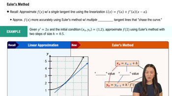 07:33
07:33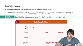 05:03
05:03Solving Initial Value Problems
Solve the initial value problems in Exercises 15–20.
t dy/dt + 2y = t³, t > 0, y(2) = 1
Use Euler’s method with dx = 0.5 to estimate y(5) if y′ = y²/√x and y(1) = −1. What is the exact value of y(5)?
Solving Initial Value Problems
Solve the initial value problems in Exercises 15–20.
θ dy/dθ + y = sin θ, θ > 0, y(π/2) = 1
Solve the Bernoulli equations in Exercises 29–32.
y' - y = xy²
What integral equation is equivalent to the initial value problem y' = f(x), y(x₀) = y₀?
Using Euler’s Method
In Exercises 15–20, use Euler’s method to calculate the first three approximations to the given initial value problem for the specified increment size. Calculate the exact solution and investigate the accuracy of your approximations. Round your results to four decimal places.
y' = 2y/x, y(1) = -1, dx = 0.5