Ch. 10 - Correlation and Regression

Triola - Elementary Statistics 14th Edition

Triola14th EditionElementary StatisticsISBN: 9780137366446Not the one you use?Change textbook

Triola 14th Edition

Ch. 10 - Correlation and Regression

Problem 10.3.12

Chapter 10, Problem 10.3.12

Interpreting a Computer Display
In Exercises 9–12, refer to the display obtained by using the paired data consisting of weights (pounds) and highway fuel consumption amounts (mi/gal) of the large cars included in Data Set 35 “Car Data” in Appendix B. Along with the paired weights and fuel consumption amounts, StatCrunch was also given the value of 4000 pounds to be used for predicting highway fuel consumption.

Finding a Prediction Interval For a car weighing 4000 pounds (x = 4000) identify the 95% prediction interval estimate of the highway fuel consumption. Write a statement interpreting that interval.

Verified step by step guidance

Step 1: Understand the problem. The goal is to identify the 95% prediction interval for a car weighing 4000 pounds (x = 4000) and interpret the interval. The prediction interval provides a range within which we expect the highway fuel consumption for a new observation to fall, with 95% confidence.

Step 2: Locate the relevant data in the computer display. From the table, the 95% prediction interval for a car weighing 4000 pounds is given as (24.634737, 33.341609). This interval is specifically labeled as '95% P.I. for new.'

Step 3: Understand the difference between a prediction interval and a confidence interval. A prediction interval accounts for both the variability in the regression model and the variability of individual observations, making it wider than a confidence interval for the mean.

Step 4: Write the interpretation of the interval. The 95% prediction interval means that we are 95% confident that the highway fuel consumption for a car weighing 4000 pounds will fall between 24.634737 mi/gal and 33.341609 mi/gal.

Step 5: Note the assumptions. The prediction interval assumes that the relationship between weight and fuel consumption is linear, the residuals are normally distributed, and the sample data is representative of the population.

Verified video answer for a similar problem:

This video solution was recommended by our tutors as helpful for the problem above.

Video duration:

Was this helpful?

Key Concepts

Here are the essential concepts you must grasp in order to answer the question correctly.

Regression Analysis

Regression analysis is a statistical method used to model the relationship between a dependent variable and one or more independent variables. In this context, it helps predict highway fuel consumption based on the weight of the car. The regression equation provided indicates how changes in weight affect fuel efficiency, allowing for predictions at specific weight values.

Prediction Interval

A prediction interval provides a range of values within which a new observation is expected to fall, with a certain level of confidence. In this case, the 95% prediction interval for a car weighing 4000 pounds indicates the range of highway fuel consumption values that can be expected for similar cars, accounting for variability in the data.

Correlation Coefficient

The correlation coefficient quantifies the strength and direction of a linear relationship between two variables. In this scenario, the negative correlation coefficient of -0.787 suggests a strong inverse relationship between car weight and fuel consumption, meaning that as weight increases, fuel efficiency tends to decrease. This information is crucial for interpreting the regression results.

Recommended video:

Guided course

05:43

Correlation Coefficient

Related Practice

Textbook Question

Finding a Prediction Interval

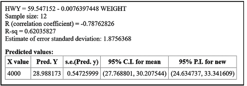
In Exercises 13–16, use the following paired data consisting of weights of large cars (pounds) and highway fuel consumption (mi/gal) from Data Set 35 “Car Data” in Appendix B. (These are the same data used in Exercises 9-12.) Let x represent the weight of the car and let y represent the corresponding highway fuel consumption. Use the given weight and the given confidence level to construct a prediction interval estimate of highway fuel consumption.

Cars Use x = 3800 pounds with a 99% confidence level.

Textbook Question

Finding the Best Model

In Exercises 5–16, construct a scatterplot and identify the mathematical model that best fits the given data. Assume that the model is to be used only for the scope of the given data, and consider only linear, quadratic, logarithmic, exponential, and power models.

Deaths from Motor Vehicle Crashes Listed below are the numbers of deaths in the United States resulting from motor vehicle crashes. Use the best model to find the projected number of such deaths for the year 2025.

Textbook Question

Regression and Predictions

Exercises 13–28 use the same data sets as Exercises 13–28 in Section 10-1.

Find the regression equation, letting the first variable be the predictor (x) variable.

Find the indicated predicted value by following the prediction procedure summarized in Figure 10-5.

Cars Sales and the Super Bowl Listed below are the annual numbers of cars sold (thousands) and the numbers of points scored in the Super Bowl that same year. What is the best predicted number of Super Bowl points in a year with sales of 8423 thousand cars? How close is the predicted number to the actual result of 37 points?

[IMAGE]

views

Textbook Question

Regression and Predictions

Exercises 13–28 use the same data sets as Exercises 13–28 in Section 10-1.

Find the regression equation, letting the first variable be the predictor (x) variable.

Find the indicated predicted value by following the prediction procedure summarized in Figure 10-5.

Taxis Use the distance/fare data from Exercise 15 and find the best predicted fare amount for a distance of 3.10 miles. How does the result compare to the actual fare of \$15.30?

Textbook Question

Appendix B Data Sets

In Exercises 29–32, use the data from Appendix B to construct a scatterplot, find the value of the linear correlation coefficient r, and find either the P-value or the critical values of r from Table A-6 using a significance level of α = 0.05. Determine whether there is sufficient evidence to support the claim of a linear correlation between the two variables.

Taxis Repeat Exercise 15 using all of the time/tip data from the 703 taxi rides listed in Data Set 32 “Taxis” from Appendix B. Compare the results to those found in Exercise 15.

Textbook Question

Best-Fit Line

What is a residual?

In what sense is the regression line the straight line that “best” fits the points in a scatterplot?