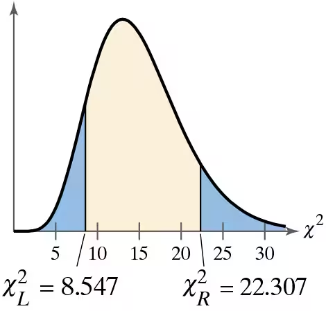
Ch. 7 - Hypothesis Testing with One Sample
Larson - Elementary Statistics: Picturing the World 8th Edition
Larson8th EditionElementary Statistics: Picturing the WorldISBN: 9780137493470Not the one you use?Change textbook
Chapter 7, Problem 7.5.14b

Graphical Analysis In Exercises 13 and 14, state whether each standardized test statistic X^2 allows you to reject the null hypothesis. Explain.


b. X^2=23.309
Graph showing a chi-squared distribution with critical values at 8.547 and 22.307, highlighting rejection regions.

Verified step by step guidance
1
Step 1: Understand the problem. The question asks whether the standardized test statistic X² = 23.309 allows you to reject the null hypothesis. To determine this, compare the test statistic to the critical values provided in the graph (X²_L = 8.547 and X²_R = 22.307).
Step 2: Recall the concept of the chi-square test. The chi-square test is used to determine whether there is a significant difference between the observed and expected frequencies in categorical data. The null hypothesis typically states that there is no difference between the observed and expected frequencies.
Step 3: Identify the rejection regions. In the graph, the rejection regions are the areas outside the critical values (X²_L = 8.547 and X²_R = 22.307). If the test statistic falls within these regions, the null hypothesis can be rejected.
Step 4: Compare the test statistic to the critical values. The test statistic X² = 23.309 is greater than the upper critical value X²_R = 22.307. This means the test statistic falls in the right-tail rejection region.
Step 5: Conclude based on the comparison. Since the test statistic is in the rejection region, you can reject the null hypothesis. This indicates that there is sufficient evidence to suggest a significant difference between the observed and expected frequencies.

Verified video answer for a similar problem:

This video solution was recommended by our tutors as helpful for the problem above.
Video duration:
2m
Was this helpful?

Key Concepts

Here are the essential concepts you must grasp in order to answer the question correctly.

Chi-Squared Distribution

The Chi-Squared distribution is a probability distribution commonly used in hypothesis testing, particularly for tests of independence and goodness-of-fit. It is characterized by its degrees of freedom, which affect its shape. The distribution is right-skewed, and as the degrees of freedom increase, it approaches a normal distribution.
Recommended video:
Guided course
07:01
Intro to Least Squares Regression

Null Hypothesis

The null hypothesis is a statement that there is no effect or no difference, and it serves as the default assumption in statistical testing. In the context of Chi-Squared tests, it often posits that observed frequencies match expected frequencies. Rejecting the null hypothesis suggests that there is sufficient evidence to support an alternative hypothesis.
Recommended video:
Guided course
06:21
Step 1: Write Hypotheses

Critical Values and Rejection Regions

Critical values are threshold points that define the boundaries of the rejection region in hypothesis testing. If the test statistic exceeds the critical value, the null hypothesis can be rejected. In the provided graph, the critical values are 8.547 and 22.307, indicating that a Chi-Squared statistic greater than 22.307 falls within the rejection region, allowing for the rejection of the null hypothesis.
Recommended video:
05:50
Critical Values: t-Distribution