In a certain region of space near Earth’s surface, a uniform horizontal magnetic field of magnitude B exists above a level defined to be y = 0. Below y = 0, the field abruptly becomes zero (Fig. 29–63). A vertical square wire loop has resistivity ρ, mass density ρm, diameter d, and side length ℓ. It is initially at rest with its lower horizontal side at y = 0 and is then allowed to fall under gravity, with its plane perpendicular to the direction of the magnetic field. (a) While the loop is still partially immersed in the magnetic field (as it falls into the zero-field region), determine the magnetic “drag” force that acts on it at the moment when its speed is υ. (b) Assume that the loop achieves a constant terminal velocity VT before its upper horizontal side exits the field. Determine a formula for VT. (c) If the loop is made of copper and B = 0.80 T, find VT.

- Ch. 01 - Introduction, Measurement, Estimating10
- Ch. 02 - Describing Motion: Kinematics in One Dimension30
- Ch. 03 - Kinematics in Two or Three Dimensions; Vectors15
- Ch. 04 - Dynamics: Newton's Laws of Motion16
- Ch. 05 - Using Newton's Laws: Friction, Circular Motion, Drag Forces22
- Ch. 06 - Gravitation and Newton's Synthesis10
- Ch. 07 - Work and Energy21
- Ch. 08 - Conservation of Energy33
- Ch. 09 - Linear Momentum26
- Ch. 10 - Rotational Motion41
- Ch. 11 - Angular Momentum; General Rotation27
- Ch. 12 - Static Equilibrium; Elasticity and Fracture27
- Ch. 13 - Fluids28
- Ch. 14 - Oscillations14
- Ch. 15 - Wave Motion35
- Ch. 16 - Sound5
- Ch. 17 - Temperature, Thermal Expansion, and the Ideal Gas Law40
- Ch. 18 - Kinetic Theory of Gases18
- Ch. 19 - Heat and the First Law of Thermodynamics31
- Ch. 20 - Second Law of Thermodynamics32
- Ch. 21 - Electric Charge and Electric Field7
- Ch. 23 - Electric Potential20
- Ch. 24 - Capacitance, Dielectrics, Electric Energy, Storage15
- Ch. 25 - Electric Current and Resistance32
- Ch. 26 - DC Circuits22
- Ch. 27 - Magnetism21
- Ch. 28 - Sources of Magnetic Field24
- Ch. 29 - Electromagnetic Induction and Faraday's Law21
- Ch. 30 - Inductance, Electromagnetic Oscillations, and AC Circuits42
- Ch. 31 - Maxwell's Equations and Electromagnetic Waves25
- Ch. 32 - Light: Reflection and Refraction42
- Ch. 33 - Lenses and Optical Instruments21
- Ch. 34 - The Wave Nature of Light: Interference and Polarization26
- Ch. 35 - Diffraction24
- Ch. 36 - The Special Theory of Relativity29
- Ch. 38 - Quantum Mechanics1
- Ch. 40 - Molecules and Solids6
- Ch. 43 - Elementary Particles3
- Ch. 44 - Astrophysics and Cosmology9
In an experiment, a coil was mounted on a low-friction cart that moved through the magnetic field B of a permanent magnet. The speed of the cart v and the induced voltage V were simultaneously measured, as the cart moved through the magnetic field, using a computer-interfaced motion sensor and a voltmeter. The Table below shows the collected data:
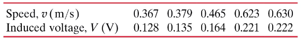
Make a graph of the induced voltage, V, vs. the speed, v. Determine a best-fit linear equation for the data. Theoretically, the relationship between V and v is given by V = BN𝓁𝓋 where N is the number of turns of the coil, B is the magnetic field, and ℓ is the average of the inside and outside widths of the coil. In the experiment, B = 0.126 T, N = 50, and ℓ = 0.0561 m.
 Verified step by step guidance
Key Concepts
Electromagnetic Induction

 05:42
05:42Linear Relationship
 07:31
07:31Graphing Data
 07:32
07:32What is the energy dissipated as a function of time in a circular loop of 18 turns of wire having a radius of 10.0 cm and a resistance of 2.0 Ω if the plane of the loop is perpendicular to a magnetic field given by B(t) = B₀e⁻ᵗ/ʳ with B₀ = 0.50 T and τ = 0.10 s?
Apply Faraday’s law, in the form of Eq. 29–8, to show that the static electric field between the plates of a parallel-plate capacitor cannot drop abruptly to zero at the edges, but must, in fact, fringe. Use the path shown dashed in Fig. 29–61. [Hint: Assume the contrary: that there is no fringing. Show that this assumption leads to a contradiction.]
In an experiment, a coil was mounted on a low-friction cart that moved through the magnetic field B of a permanent magnet. The speed of the cart v and the induced voltage V were simultaneously measured, as the cart moved through the magnetic field, using a computer-interfaced motion sensor and a voltmeter. The Table below shows the collected data:
Find the % error between the slope of the experimental graph and the theoretical value for the slope.