Ch. 9 - First-Order Differential Equations
Hass - Thomas' Calculus 15th Edition
Hass15th EditionThomas' CalculusISBN: 9780137616077Not the one you use?Change textbook
Chapter 9, Problem 9.1.41

In Exercises 39–42, use Euler’s method with the specified step size to estimate the value of the solution at the given point x*. Find the value of the exact solution at x*.


y′ = √x/y, y > 0, y(0) = 1, dx = 0.1, x* = 1

Verified step by step guidance
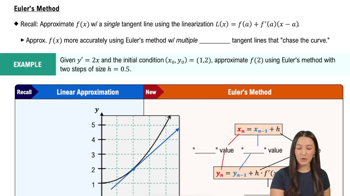
1
Identify the differential equation and initial condition: \(y' = \frac{\sqrt{x}}{y}\) with \(y(0) = 1\).
Set the step size \(\Delta x = 0.1\) and the target point \(x^* = 1\). Determine the number of steps needed: \(n = \frac{x^* - 0}{\Delta x} = 10\) steps.
Apply Euler's method iteratively using the formula: \(y_{k+1} = y_k + \Delta x \cdot f(x_k, y_k)\), where \(f(x, y) = \frac{\sqrt{x}}{y}\).
Start with \(x_0 = 0\) and \(y_0 = 1\). For each step \(k\) from 0 to 9, compute \(y_{k+1}\) using the formula and update \(x_{k+1} = x_k + \Delta x\).
To find the exact solution at \(x^* = 1\), solve the differential equation analytically by separating variables and applying the initial condition, then evaluate the solution at \(x = 1\).

Verified video answer for a similar problem:

This video solution was recommended by our tutors as helpful for the problem above.
Video duration:
10m
Was this helpful?

Key Concepts

Here are the essential concepts you must grasp in order to answer the question correctly.

Euler's Method

Euler's method is a numerical technique to approximate solutions of first-order differential equations. It uses a step size to incrementally estimate the function's value by moving along the slope given by the differential equation. This method is especially useful when an exact solution is difficult to find.
Recommended video:
07:33
Euler's Method

Initial Value Problems (IVP)

An initial value problem specifies the value of the solution at a starting point, allowing the differential equation to be solved uniquely. Here, y(0) = 1 sets the initial condition, which is essential for applying Euler's method and finding the particular solution.
Recommended video:
05:03
Initial Value Problems

Exact Solution of Differential Equations

The exact solution is an explicit formula that satisfies the differential equation and initial condition. Finding it involves techniques like separation of variables or integration. Comparing the exact solution to the Euler approximation helps assess the accuracy of the numerical method.
Recommended video:
04:00
Solutions to Basic Differential Equations
Related Practice
Textbook Question

Integral Equations

In Exercises 7–12, write an equivalent first-order differential equation

and initial condition for y.


y = ln x + ∫ₓᵉ √ (t² + (y(t))²) dt

Textbook Question

First-Order Linear Equations

Solve the differential equations in Exercises 1–14.


tan θ dr/dθ + r = sin²θ, 0 < θ < π/2

Textbook Question

Carbon monoxide pollution An executive conference room of a corporation contains 4500 ft³ of air initially free of carbon monoxide. Starting at time t = 0, cigarette smoke containing 4% carbon monoxide is blown into the room at the rate of 0.3 ft³/min. A ceiling fan keeps the air in the room well circulated and the air leaves the room at the same rate of 0.3 ft³/min. Find the time when the concentration of carbon monoxide in the room reaches 0.01%.

1
views
Textbook Question

In Exercises 39–42, use Euler’s method with the specified step size to estimate the value of the solution at the given point x*. Find the value of the exact solution at x*.


y' = 2xexp(x²) , y(0) = 2, dx = 0.1, x* = 1

Textbook Question

Using Euler’s Method

In Exercises 15–20, use Euler’s method to calculate the first three approximations to the given initial value problem for the specified increment size. Calculate the exact solution and investigate the accuracy of your approximations. Round your results to four decimal places.


y' = x(1-y), y(1) = 0, dx = 0.2

Textbook Question

Write the formula for a logistic function that has values between y = 0 and y = 1, crosses the line y = 1/2 at x = 0, and has slope 5 at this point.