Textbook Question
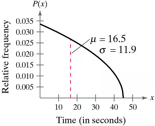
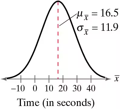
Graphical Analysis In Exercises 17–22, find the indicated z-score(s) shown in the graph.
" style="" width="260">
 Verified step by step guidance
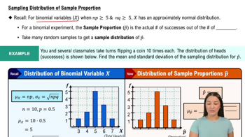
 05:11
05:11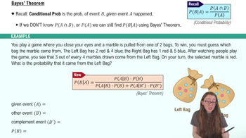 05:10
05:10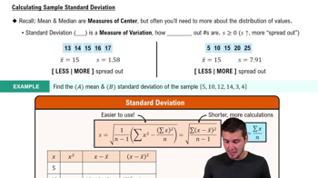 08:45
08:45Graphical Analysis In Exercises 17–22, find the indicated z-score(s) shown in the graph.
" style="" width="260">
Finding Probabilities In Exercises 15–18, the population mean and standard deviation are given. Find the indicated probability and determine whether the given sample mean would be considered unusual.
For a random sample of n=36, find the probability of a sample mean being less than 12,750 or greater than 12,753 when mu=12750 and 1.7.
Computing and Interpreting z-Scores In Exercises 39 and 40, (a) find the z-score that corresponds to each value and (b) determine whether any of the values are unusual.
Stanford-Binet IQ Scores The test scores for the Stanford-Binet Intelligence Scale are normally distributed with a mean score of 100 and a standard deviation of 16. The test scores of four students selected at random are 98, 65, 106, and 124.
Finding Area
In Exercises 23–36, find the indicated area under the standard normal curve. If convenient, use technology to find the area.
To the left of z=0.33
In Exercises 1–4, a population has a mean mu and a standard deviation sigma. Find the mean and standard deviation of the sampling distribution of sample means with sample size n.
Mu = 150, sigma =25, n = 49
Construction About 63% of the residents in a town are in favor of building a new high school. One hundred five residents are randomly selected. What is the probability that the sample proportion in favor of building a new school is less than 55%? Interpret your result.