

 10:17
10:17
Textbook Question
Performing a Chi-Square Goodness-of-Fit Test
In Exercises 7–16, (a) identify the claim and state H₀ and Hₐ.
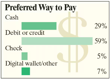
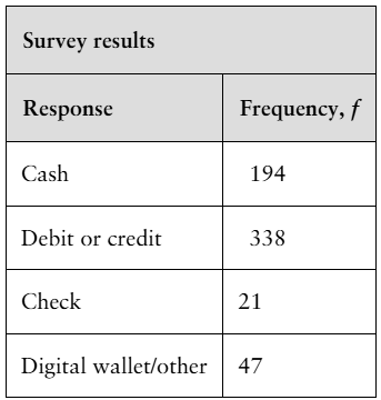
Ways to Pay A financial analyst claims that the distribution of people’s preferences on how to pay for goods is different from the distribution shown in the figure. You randomly select 600 people and record their preferences on how to pay for goods. The table shows the results. At α=0.01, test the financial analyst’s claim. (Adapted from Travis Credit Union)