
Textbook Question
Integral Equations
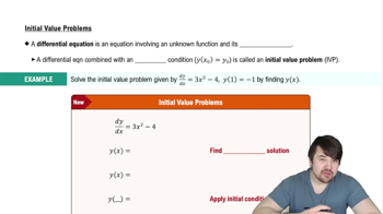
In Exercises 7–12, write an equivalent first-order differential equation
and initial condition for y.
y = ln x + ∫ₓᵉ √ (t² + (y(t))²) dt

 Verified step by step guidance
 07:33
07:33
 05:03
05:03 04:57
04:57Integral Equations
In Exercises 7–12, write an equivalent first-order differential equation
and initial condition for y.
y = ln x + ∫ₓᵉ √ (t² + (y(t))²) dt
Carbon monoxide pollution An executive conference room of a corporation contains 4500 ft³ of air initially free of carbon monoxide. Starting at time t = 0, cigarette smoke containing 4% carbon monoxide is blown into the room at the rate of 0.3 ft³/min. A ceiling fan keeps the air in the room well circulated and the air leaves the room at the same rate of 0.3 ft³/min. Find the time when the concentration of carbon monoxide in the room reaches 0.01%.
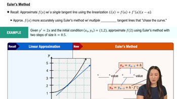
In Exercises 39–42, use Euler’s method with the specified step size to estimate the value of the solution at the given point x*. Find the value of the exact solution at x*.
y' = 2xexp(x²) , y(0) = 2, dx = 0.1, x* = 1
Write the formula for a logistic function that has values between y = 0 and y = 1, crosses the line y = 1/2 at x = 0, and has slope 5 at this point.
Use Euler’s method with dx = 0.2 to estimate y(1) if y′ = y and y(0) = 1. What is the exact value of y(1)?
In Exercises 39–42, use Euler’s method with the specified step size to estimate the value of the solution at the given point x*. Find the value of the exact solution at x*.
y' = 2y²(x-1), y(2) = -1/2, dx = 0.1, x* = 3