Ch. 9 - Differential Equations
Briggs - Calculus: Early Transcendentals 3rd Edition
Briggs3rd EditionCalculus: Early TranscendentalsISBN: 9780136847243Not the one you use?Change textbook
Chapter 9, Problem 9.R.20b

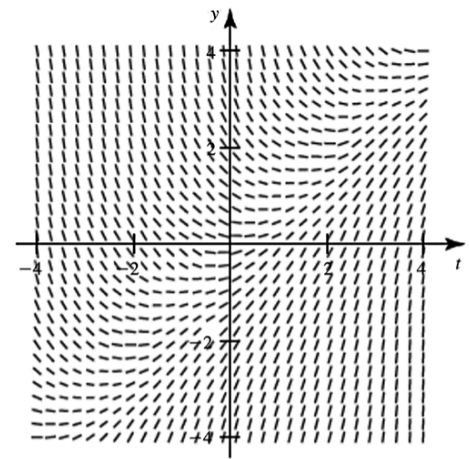
Direction fields The direction field for the equation y′(t)=t−y, for |t|≤4 and |y|≤4, is shown in the figure.
b. Use the direction field to sketch the solution curve that passes through the point (0,−1/2).
Direction field plot showing slope vectors for y′(t) = t minus y over t and y from -4 to 4.

Verified step by step guidance
1
Identify the initial point given in the problem, which is (0, -\(\frac{1}{2}\)). This is where your solution curve will start on the direction field.
At the initial point, observe the slope of the direction field. The slope is given by the differential equation y\'(t) = t - y. Substitute t = 0 and y = -\(\frac{1}{2}\) into the equation to find the slope at this point: y\'(0) = 0 - (-\(\frac{1}{2}\)) = \(\frac{1}{2}\).
Using the slope \(\frac{1}{2}\) at the initial point, sketch a small line segment starting at (0, -\(\frac{1}{2}\)) that rises gently, reflecting this positive slope.
Follow the direction field arrows from the initial point, moving step-by-step along the slopes indicated by the field. At each new point, estimate the slope from the nearby direction field vectors and continue drawing the curve smoothly, ensuring it aligns with the slope directions.
Continue this process both forward and backward in t, making sure the curve remains consistent with the slope directions shown in the direction field, thus sketching the solution curve that passes through (0, -\(\frac{1}{2}\)).

Verified video answer for a similar problem:

This video solution was recommended by our tutors as helpful for the problem above.
Video duration:
2m
Was this helpful?

Key Concepts

Here are the essential concepts you must grasp in order to answer the question correctly.

Direction Fields (Slope Fields)

A direction field is a graphical representation of a first-order differential equation showing small line segments with slopes given by the differential equation at various points. It helps visualize the behavior of solutions without solving the equation analytically. Each segment indicates the slope of the solution curve passing through that point.
Recommended video:
05:45
Understanding Slope Fields

Initial Value Problem and Solution Curves

An initial value problem specifies a differential equation along with a point through which the solution curve must pass. Using the direction field, one can sketch the solution curve starting at the initial point by following the slope directions, illustrating how the solution evolves over the domain.
Recommended video:
05:03
Initial Value Problems

Differential Equation y′(t) = t − y

This equation defines the slope of the solution curve at any point (t, y) as the difference between t and y. Understanding how the slope depends on both variables is crucial for interpreting the direction field and predicting the shape of solution curves, especially near the initial condition.
Recommended video:
07:39
Classifying Differential Equations