Textbook Question
Area by geometry Use geometry to evaluate the following definite integrals, where the graph of ƒ is given in the figure.
(a) ∫₀⁴ ƒ(𝓍) d𝓍
1
views

 Verified step by step guidance
 06:21
06:21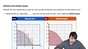 05:43
05:43 06:18
06:18Area by geometry Use geometry to evaluate the following definite integrals, where the graph of ƒ is given in the figure.
(a) ∫₀⁴ ƒ(𝓍) d𝓍
Approximating areas Estimate the area of the region bounded by the graph of ƒ(𝓍) = x² + 2 and the x-axis on [0, 2] in the following ways.
(a) Divide [0, 2] into n = 4 subintervals and approximate the area of the region using a left Riemann sum. Illustrate the solution geometrically.
The velocity in ft/s of an object moving along a line is given by v = ƒ(t) on the interval 0 ≤ t ≤ 6 (see figure), where t is measured in seconds.
(a) Divide the interval [0,6] into n = 3 subintervals, [0,2] , [2,4] and [4,6]. On each subinterval, assume the object moves at a constant velocity equal to the value of v evaluated at the right endpoint of the subinterval, and use these approximations to estimate the displacement of the object on [0,6] (see part (a) of the figure)
Sigma notation Evaluate the following expressions.
(a) 10
∑ κ
κ=1
Symmetry properties Suppose ∫₀⁴ ƒ(𝓍) d𝓍 = 10 and ∫₀⁴ g(𝓍) d𝓍 = 20. Furthermore, suppose ƒ is an even function and g is an odd function. Evaluate the following integrals.
(a) ∫₋₄⁴ ƒ(𝓍) d𝓍
Symmetry properties Suppose ∫₀⁴ ƒ(𝓍) d𝓍 = 10 and ∫₀⁴ g(𝓍) d𝓍 = 20. Furthermore, suppose ƒ is an even function and g is an odd function. Evaluate the following integrals.
(c) ∫₋₄⁴ (4ƒ(𝓍) ― 3g(𝓍))d𝓍